Page 95 - 2024-bfw-starnes-TPS7e-SE proofs.indd

82 UNIT 1 Exploring One-Variable Data

(a) Make a dotplot to display the data.
35
32% (b) What proportion of this group of students remem-

30
bered 20 or more words?
25 (c) Find the median of the distribution.
20%
Percent 15 13% 13% (d) Is the mean of the distribution less than, about the
20

© 2024 BFW Publishers PAGES NOT FINAL - For Review Purposes Only - Do Not Copy
same as, or greater than the median? Explain how you
10 know without performing any calculations.
5
R6 Density of the earth (1C, 1D) In 1798, the English
0 scientist Henry Cavendish measured the density of
YouTube Snapchat TikTok Instagram
Site you don’t want to live without the earth several times by careful work with a torsion
balance. The variable recorded was the density of the
earth as a multiple of the density of water. Here are
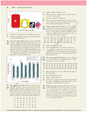
(a) Explain how the graph gives a misleading impression. Cavendish’s 29 measurements: 96
(b) Would it be appropriate to make a pie chart to display

the data? Why or why not? 5.50 5.61 4.88 5.07 5.26 5.55 5.36 5.29 5.58 5.65
5.57 5.53 5.62 5.29 5.44 5.34 5.79 5.10 5.27 5.39
R4 Success in college (1B) A national survey asked 95,505
first-year college students about specific academic 5.42 5.47 5.63 5.34 5.46 5.30 5.75 5.68 5.85
behaviors identified by college faculty as being import-
ant for student success. One question asked, “How often (a) Make a stemplot of the data.

in the past year did you ask questions during class?” The (b) Describe the distribution of density measurements.
figure is a side-by-side bar graph comparing the percent- (c) The currently accepted value for the density of the
age who answered “frequently” by race/ ethnic group earth is 5.51 times the density of water. How does this
and whether the respondent was a first- generation col- value compare to the mean of the distribution of den-
94

lege student. Describe what you see. sity measurements?
First-generation R7 Eat your oatmeal (1C, 1D) Researchers collected
60 Not first-generation data on the calories in 39 different brands of single-
54.4 48.3 45.8 48.6 46.9 44.5 44.5 46.1 serve oatmeal. Here are the data: 97
Percentage of students 50 38.8 38.7 31.3 36.5 36.4 40.7 100 110 130 130 140 150 150 150 150 160 160 160 160

40
170 170 170 170 170 180 190 190 200 200 210 210 210
210 220 220 230 230 240 240 250 270 280 300 310 350
30
20
the distribution.
10 (a) Make a histogram of the data. Describe the shape of
(b) Find the interquartile range.
0 (c) Make a boxplot of the data.
American Asian Black Hispanic White Other Two or

Indian more races (d) Compare the histogram from part (a) with the boxplot
Race/ethnicity from part (c). Identify an aspect of the distribution that
one graph reveals but the other does not.

R5 Music and memory (1C, 1D) For a final project in R8 High versus low incomes (1C) Rich and poor
®
their AP Statistics class, two students studied the households differ in ways that go beyond income.
impact of different types of background music on stu- Here are histograms that compare the distribu-
dents’ ability to remember words from a list they were tions of household size (number of people) for
allowed to study for 5 minutes. Here are data on the low- income and high- income households. Low-
98

number of words remembered by one group of stu- income households had annual incomes less than
dents who listened to Beethoven’s Fifth Symphony: 95 $15,000, and high-income households had annual
incomes of at least $100,000.
11 12 23 15 14 15 14 15
10 14 15 9 11 13 25 11
13 13 12 20 17 23 11 12
12 11 20 20 12 12 19 13
15 10 14 11 7 17 13 18

© 2024 BFW Publishers PAGES NOT FINAL - For Review Purposes Only, all other uses prohibited - Do Not Copy or Post in Any Form.

02_StarnesTPS7e_40934_un01_p1_001_086_6pp.indd 82 13/09/23 5:40 PM