Page 90 - 2024-bfw-starnes-TPS7e-SE proofs.indd

P. 90

SecTIoN 1D Exercises 77

(a) From the boxplots, what can you say about the percent-
age of people in each of the three dieting groups who
lost less than 5% of their body weight?
0 5 10 15 20 25 30 35 40
(b) Compare the distributions of percentage of body Number of pairs of shoes
weight lost for the three dieting groups.
© 2024 BFW Publishers PAGES NOT FINAL - For Review Purposes Only - Do Not Copy
39. On-site worker commutes How long do on-site work- (a) Calculate the mean of the distribution.
ers typically spend traveling to their workplace? The (b) Calculate the 10% trimmed mean.
answer may depend on where they live. Here are the
travel times (in minutes) of 20 randomly chosen on-site (c) Why is the trimmed mean a better summary of the
workers in New York state and 15 randomly chosen center of this distribution than the mean?
on-site workers in North Carolina: 90
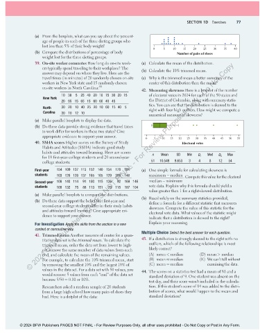
42. Measuring skewness Here is a boxplot of the number
10 30 5 25 40 20 10 15 30 20 15 of electoral votes in 2024 for each of the 50 states and
New York
20 85 15 65 15 60 60 40 45 the District of Columbia, along with summary statis-
tics. You can see that the distribution is skewed to the
North 30 20 10 40 25 20 10 60 15 40 5 right with four high outliers. How might we compute a
Carolina 30 10 12 10 numerical measure of skewness?
(a) Make parallel boxplots to display the data.
(b) Do these data provide strong evidence that travel times
to work differ for workers in these two states? Give
appropriate evidence to support your answer.
0 5 10 15 20 25 30 35 40 45 50 55
40. SSHA scores Higher scores on the Survey of Study Electoral votes
Habits and Attitudes (SSHA) indicate good study
habits and attitudes toward learning. Here are scores n Mean SD Min Med Max
for 18 first-year college students and 20 second-year Q 1 Q 3
college students: 51 10.549 9.653 3 4 8 12 54

First-year 154 109 137 115 152 140 154 178 101 (a) One simple formula for calculating skewness is
students 103 126 126 137 165 165 129 200 148 maximum −median . Compute this value for the electoral
Second-year 108 140 114 91 180 115 126 92 169 146 median −minimum
students 109 132 75 88 113 151 70 115 187 104 vote data. Explain why this formula should yield a
value greater than 1 for a right-skewed distribution.
(a) Make parallel boxplots to compare the distributions.
(b) Do these data support the belief that first-year and (b) Based solely on the summary statistics provided,
define a formula for a different statistic that measures
second-year college students differ in their study habits skewness. Compute the value of this statistic for the
and attitudes toward learning? Give appropriate evi- electoral vote data. What values of the statistic might
dence to support your answer.
indicate that a distribution is skewed to the right?
For Investigation Apply the skills from the section in a new Explain your reasoning.
context or nonroutine way.
Multiple Choice Select the best answer for each question.
41. Trimmed mean Another measure of center for a quan-
titative data set is the trimmed mean. To calculate the 43. If a distribution is strongly skewed to the right with no
trimmed mean, order the data set from lowest to high- outliers, which of the following relationships is most
est, remove the same number of data values from each likely correct?
end, and calculate the mean of the remaining values. (A) mean < median (D) mean > median
For example, to calculate the 10% trimmed mean, start (B) mean ≈ median (E) We can’t tell without
by removing the smallest 10% and the largest 10% of (C) mean = median examining the data.
values in the data set. For a data set with 50 values, you 44. The scores on a statistics test had a mean of 81 and a
would remove 5 values from each “end” of the data set standard deviation of 9. One student was absent on the
because 5/50 = 0.10 or 10%. test day, and their score wasn’t included in the calcula-
Researchers asked a random sample of 20 students tion. If this student’s score of 84 was added to the distri-
from a large high school how many pairs of shoes they bution of scores, what would happen to the mean and
had. Here is a dotplot of the data: standard deviation?

02_StarnesTPS7e_40934_un01_p1_001_086_6pp.indd 77 13/09/23 5:40 PM

85 86 87 88 89 90 91 92 93 94 95