Page 58 - 2024-bfw-starnes-TPS7e-SE proofs.indd

SecTIoN 1c Exercises 45

(b) According to the World Health Organization, a person
with a BMI less than 18 is considered underweight. 22
20
Compare the percentages of rural and semi-urban 18
women in the sample who are underweight. 16

34. Paper towels In commercials for Bounty paper 14
© 2024 BFW Publishers PAGES NOT FINAL - For Review Purposes Only - Do Not Copy
towels, the manufacturer claims that they are the Frequency 12
“quicker picker-upper”—but are they also the 10 8
stronger picker-upper? Two statistics students decided 6
to investigate. They selected a random sample of 4
30 Bounty paper towels and a random sample of 30 2
generic paper towels and measured their strength 0
when wet. To do this, the students uniformly soaked 70 75 80 85 90 95 100
each paper towel with 4 ounces of water, held two Percentage wearing seat belts
opposite edges of the paper towel, and counted how
many quarters each paper towel could hold until rip- (a) In what proportion of states was at least 90% seat belt
ping. The data are displayed in the relative frequency use observed?
histograms. 57 (b) Describe the shape of the distribution.
Thirty-four states enforce a seat belt violation as a pri-
30 mary offense, while 16 states enforce a seat belt viola-
Bounty
Relative frequency (%) 10 0 the percentage of people who were wearing seat belts
tion only as a secondary offense. The histograms show
20
in primary enforcement versus secondary enforcement
states during the NHTSA study.
30
Generic
20
10 0.35 Primary
0.30
0
76 88 100 112 124 136 0.25
Number of quarters Relative frequency 0.20

(a) Describe similarities and differences between the two 0.15
distributions. 0.10
(b) What conclusion should the students make from their 0.05
research? Explain your answer. 0.00
70 75 80 85 90 95 100
35. Birth months Imagine asking a random sample of 60 Percentage wearing seat belts
students from your school about their birth months.
Draw a plausible (believable) graph of the distribution 0.35 Secondary
of birth month. Should you use a bar graph or a histo-
gram to display the data? 0.30

36. Die rolls Imagine rolling a fair, six-sided die 60 times. 0.25
Draw a plausible (believable) graph of the distribution Relative frequency 0.20
of die rolls. Should you use a bar graph or a histogram 0.15
to display the data? 0.10
37. Seat belts Each year, the National Highway Traffic 0.05
Safety Administration (NHTSA) conducts an obser- 0.00
vational study of seat belt use in all 50 states. Trained 70 75 80 85 90 95 100
observers station themselves at randomly selected Percentage wearing seat belts
locations along roadways in each state, and then record
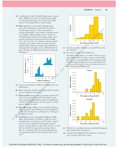
data on seat belt use by people in passing vehicles. (c) Why did we use relative frequency instead of frequency
Here is a histogram of the percentage of people who when making these histograms?
were wearing seat belts in each state during a recent (d) Compare the distributions of seat belt use in primary
year: 58 and secondary enforcement states.

© 2024 BFW Publishers PAGES NOT FINAL - For Review Purposes Only, all other uses prohibited - Do Not Copy or Post in Any Form.

02_StarnesTPS7e_40934_un01_p1_001_086_6pp.indd 45 13/09/23 5:38 PM