Page 61 - 2024-bfw-starnes-TPS7e-SE proofs.indd

48 UNIT 1 Exploring One-Variable Data

SECTION 1D Describing Quantitative Data
with Numbers

© 2024 BFW Publishers PAGES NOT FINAL - For Review Purposes Only - Do Not Copy
LEARNING TARGETS By the end of the section, you should be able to:

• Find the median of a distribution of quantitative data. • Choose appropriate measures of center and

• Calculate the mean of a distribution of quantitative variability to summarize a distribution of

data. quantitative data.

• Find the range of a distribution of quantitative data. • Identify outliers in a distribution of quantitative

• Calculate and interpret the standard deviation of a data.

distribution of quantitative data. • Make and interpret boxplots of quantitative data.

• Find the interquartile range ( IQR ) of a distribution of • Use boxplots and summary statistics to compare
quantitative data. distributions of quantitative data.
In Section 1C, you learned how to display quantitative data with graphs. You
also explored how to use these graphs to describe and compare distributions of
a quantitative variable. In this section, we’ll focus on numerical summaries of
quantitative data.
Let’s return to a familiar context from the preceding section. Recall that city
managers in Flint, Michigan, switched the city’s water source from Lake Huron
to the Flint River to save money. Here once again are the lead levels (in parts per
billion, ppb) in 71 water samples collected from randomly selected Flint dwell-

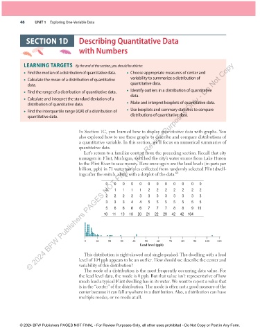
ings after the switch, along with a dotplot of the data . 64
0 0 0 0 0 0 0 0 0 0 0 0
0 1 1 1 1 2 2 2 2 2 2 2
2 2 2 2 3 3 3 3 3 3 3 3
3 3 3 4 4 5 5 5 5 5 5 5
5 6 6 6 6 7 7 7 8 8 9 10
10 11 13 18 20 21 22 29 42 42 104

0 10 20 30 40 50 60 70 80 90 100 110
Lead level (ppb)
This distribution is right-skewed and single-peaked. The dwelling with a lead
level of 104 ppb appears to be an outlier. How should we describe the center and
variability of this distribution?
The mode of a distribution is the most frequently occurring data value. For
the lead level data, the mode is 0 ppb. But that value isn’t representative of how
much lead a typical Flint dwelling has in its water. We want to report a value that
is in the “center” of the distribution. The mode is often not a good measure of the
center because it can fall anywhere in a distribution. Also, a distribution can have
multiple modes, or no mode at all.

© 2024 BFW Publishers PAGES NOT FINAL - For Review Purposes Only, all other uses prohibited - Do Not Copy or Post in Any Form.

02_StarnesTPS7e_40934_un01_p1_001_086_6pp.indd 48 13/09/23 5:38 PM