Page 43 - 2024-bfw-starnes-TPS7e-SE proofs.indd

30 UNIT 1 Exploring One-Variable Data

EXAMPLE Preventing concussions Skills 2.A, 2.B
Displaying quantitative data: Stemplots

PROBLEM: Many athletes (and their parents) worry about the risk of con-

cussions when playing sports. A youth football coach plans to obtain spe-
© 2024 BFW Publishers PAGES NOT FINAL - For Review Purposes Only - Do Not Copy
cially made helmets for the players that are designed to reduce their chance
of getting a concussion. Here are the measurements of head circumference
(in inches) for the 30 players on the team: 35
23.0 22.2 21.7 22.0 22.3 22.6 22.7 21.5 22.7 25.6
20.8 23.0 24.2 23.5 20.8 24.0 22.7 22.6 23.9 22.5
Pete Saloutos/AGE Fotostock
23.1 21.9 21.0 22.4 23.5 22.5 23.9 23.4 21.6 23.3
(a) Make a stemplot of these data.

(b) Describe the shape of the distribution. Are there any obvious outliers?
SOLUTION:
( a) 20 88 To make the stemplot:
21 05679 Key: 23|5 is a 1. Make stems. The smallest head circumference is 20.8 inches and the largest

player with
22 02345566777 is 25.6 inches. We use the first two digits as the stem and the final digit as the
23 001345599 a head leaf. So we need stems from 20 to 25.
circumference
24 02 of 23.5 inches.
25 6 2. Add leaves. For the player with a head circumference of 23.0 inches, place a 0 on
the 23 stem. For the player with a head circumference of 22.2 inches, place a 2 on
the 22 stem. Continue in this way until you have added the data for all the players.
(b) The distribution of head circum- 3. Order the leaves.
ference for the 30 players on the 4. Add a key.
youth football team is roughly
symmetric, with a single peak on the 22-inch stem.
There are no obvious outliers.
FoR PRAcTIce, TRY eXeRcISe 17

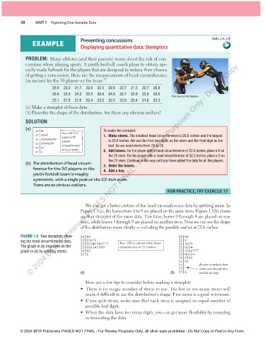
We can get a better picture of the head circumference data by splitting stems. In
Figure 1.5(a) , the leaves from 0 to 9 are placed on the same stem. Figure 1.5(b) shows

another stemplot of the same data. This time, leaves 0 through 4 are placed on one
stem, while leaves 5 through 9 are placed on another stem. Now we can see the shape
of the distribution more clearly — including the possible outlier at 25.6 inches.

FIGURE 1.5 Two stemplots show- 20 88 20 88
ing the head circumference data. 21 05679 Key: 23|5 is a player with a head 21 0
The graph in (b) improves on the 22 02345566777 circumference of 23.5 inches. 21 5679
22 0234
23 001345599
graph in (a) by splitting stems. 24 02 22 5566777
25 6 23 00134
23 5599
24 02
24 Be sure to include these
25 stems even though they
(a) (b) 25 6 include no data.
Here are a few tips to consider before making a stemplot:

• There is no magic number of stems to use. Too few or too many stems will

make it difficult to see the distribution’s shape. Five stems is a good minimum.

• If you split stems, make sure that each stem is assigned an equal number of
possible leaf digits.
• When the data have too many digits, you can get more flexibility by rounding

or truncating the data.

© 2024 BFW Publishers PAGES NOT FINAL - For Review Purposes Only, all other uses prohibited - Do Not Copy or Post in Any Form.

02_StarnesTPS7e_40934_un01_p1_001_086_6pp.indd 30 13/09/23 5:37 PM