Page 72 - 2024-calc4e-SE proofs-4e.indd

Sullivan 04 apcalc4e 45342 ch02 166 233 5pp August 7, 2023 12:54

222 Chapter 2 • The Derivative and Its Properties

Application: Simple Harmonic Motion

Simple harmonic motion is a repetitive motion that can be modeled by a
trigonometric function. A swinging pendulum and an oscillating spring are examples
of simple harmonic motion.

EXAMPLE 6 Analyzing Simple Harmonic Motion
length l of the spring after t seconds is modeled by the function l(t) = 2 + cos t.Copy.
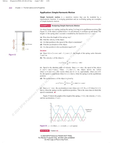
An object hangs on a spring, making the spring 2 m long in its equilibrium position. See
Figure 32. If the object is pulled down 1 m and released, it oscillates up and down. The
© 2024 BFW Publishers PAGES NOT FINAL - For Review Purposes Only - Do Not

(a) How does the length of the spring vary?
1 (b) Find the velocity of the object.
(c) At what position is the speed of the object a maximum?
Equ
2 Equilibrium (d) Find the acceleration of the object.
(e) At what position is the acceleration equal to 0?
t
3 t  0
Solution
(a) Since l(t) = 2 + cos t and −1 ≤ cos t ≤ 1, the length of the spring varies between
Figure 32
1 and 3 m.
(b) The velocity v of the object is
d
′
v =l (t) = (2 + cos t) = −sin t
dt
(c) Speed is the absolute value of velocity. Since v = −sin t, the speed of the object
is |v| = |−sin t| = |sin t| . Since −1 ≤ sin t ≤ 1, the object moves the fastest
when |v| = |sin t| = 1. This occurs when sin t = ±1 or, equivalently, when cos t = 0.
So, the speed is a maximum when l(t) = 2, that is, when the spring is at the equilibrium
position.
(d) The acceleration a of the object is given by

d d
′′ ′
a =l (t) = l (t) = (−sin t) = −cos t
dt dt
(e) Since a = −cos t, the acceleration is zero when cos t = 0. So, a = 0 when l(t) = 2,
that is, when the spring is at the equilibrium position. This is the same time at which the
speed is maximum.

Figure 33 shows the graphs of the length of the spring y =l(t), the velocity y = v(t),
and the acceleration y = a(t).

y
3 y l(t)

2 Equilibrium
position
1

t
1 y a(t) y v(t)

Figure 33 y = l(t)(blue), y = v(t)(red), y = a(t)(green)

NOW WORK Problem 65.

© 2024 BFW Publishers PAGES NOT FINAL
For Review Purposes Only, all other uses prohibited
Do Not Copy or Post in Any Form.