Page 67 - 2024-bfw-starnes-TPS7e-SE proofs.indd

54 UNIT 1 Exploring One-Variable Data

CHECK YOUR
UNDERSTANDING

Some students purchased pumpkins for a carving contest. Before the contest began,
they weighed the pumpkins. The weights (in pounds) are shown here, along with a
© 2024 BFW Publishers PAGES NOT FINAL - For Review Purposes Only - Do Not Copy
histogram of the data.
8
3.6 4.0 9.6 14.0 11.0
7
12.4 13.0 2.0 6.0 6.6
15.0 3.4 12.7 6.0 2.8 Frequency 6 5
9.6 4.0 6.1 5.4 11.9 4 3
5.4 31.0 33.0 2
1
0
0 5 10 15 20 25 30 35
Pumpkin weight (lb)
1. Find the median weight of the pumpkins.

2. Calculate the mean weight of the pumpkins.

3. Explain why the mean of the distribution would be larger than the median
before doing any calculations.

Measuring Variability: The Range

Being able to describe the shape and center of a distribution of quantitative data
is a great start. However, two distributions can have the same shape and center,
but still look quite different.

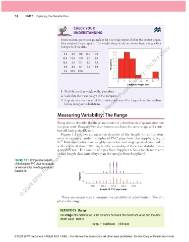
Figure 1.11 shows comparative dotplots of the length (in millimeters,
mm) of separate random samples of PVC pipe from two suppliers, A and
67
B. Both distributions are roughly symmetric and single-peaked (unimodal),
with centers at about 600 mm, but the variability of these two distributions is
quite different. The sample of pipes from Supplier A has a much more con-
sistent length (less variability) than the sample from Supplier B.

FIGURE 1.11 Comparative dotplots
of the length of PVC pipes in separate
random samples from Supplier A and
Supplier B.
Supplier A

B
597.0 598.5 600.0 601.5 603.0
Length of PVC pipe (mm)

There are several ways to measure the variability of a distribution. The sim-
plest is the range.

DEFINITION Range
The range of a distribution is the distance between the minimum value and the max-
imum value. That is,
−
range = maximumminimum

© 2024 BFW Publishers PAGES NOT FINAL - For Review Purposes Only, all other uses prohibited - Do Not Copy or Post in Any Form.

02_StarnesTPS7e_40934_un01_p1_001_086_6pp.indd 54 13/09/23 5:38 PM